A study that has finished collecting sits in an awkward position. The sessions are there, but the first questions asked of them are usually small: did the manipulation move reaction times at all, how many participants completed every block, is the condition variable actually populated. The standard route to an answer is to export a CSV and open R. That round trip is the right one for the analysis that goes into the paper. It is heavy for the questions that come before it.
Open Lab has two places where collected data can be looked at, and they are built for different points in that sequence. This post sets out what each one does, which datasets each one can see, and where the limits sit. The reference documentation covers the same ground in a different form: Data Analysis for the per-study view and Data Explorer for the query workspace.
The two surfaces do different jobs
The Data view belongs to a single study. It is reached from the study dashboard by clicking the "Data Collected" card, and there is a parallel view on a Task that aggregates across every study using that task. It refreshes every 30 seconds, so it is the view to keep open while collection is running. It lists the datasets in a filterable, sortable table, charts responses over time and per day, reports summary statistics, shows a participant-inactivity breakdown, holds the controls for decrypting an encrypted study, and provides the exports.
The exports are gated by plan, which is worth knowing before planning an analysis around a particular format:
| Export | Plan |
|---|---|
| Individual responses (CSV) · Response statistics (CSV) | Free and above |
| JSON · Excel (.xlsx) | Basic and above |
| Wide-format CSV · SPSS (.sav) | Pro and above |
| PDF report | Team and above |
The Data Explorer is account-level rather than study-level. It opens from the Data Explorer link
in the dashboard sidebar, at /dashboard/analysis. Its left panel lists the studies you own and the
studies shared with you through a project, you select one or more, and Load Data pulls their trial
data into the browser. A short tour runs the first time and can be dismissed.
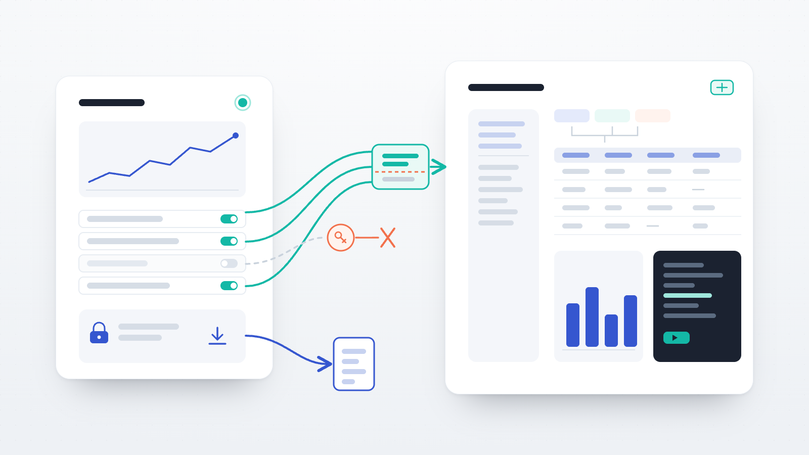
So the division is roughly: the Data view is for monitoring one study, decrypting it, and getting the data out; the Data Explorer is for asking questions of data from one or several studies without getting it out first.
What loading data actually does
Every trial event in the selected studies is flattened into one table called trials, with one row
per event. Each row carries the columns your task recorded, plus nine metadata columns written by
the platform and prefixed with an underscore so they do not collide with your own variable names:
_study_id, _study_title, _task_title, _participant_code, _stable_id, _group_code,
_session_id, _dataset_id and _completed_at.
Two of those are more useful than they look. _group_code carries the between-subjects condition
assigned at the landing page, so a between-subjects comparison is a split by away without
touching the task data. _stable_id identifies a returning participant across sessions, which is
what a repeated-measures grouping needs.
Because several studies land in the same table, a column present in one study and absent in another is null for the rows that came from the other. That is what makes combining replications straightforward, and it is also the first thing to check in the schema panel if a query returns fewer rows than expected.
The table lives in DuckDB compiled to WebAssembly and running inside the browser tab. Queries execute on your own machine; the data does not travel to a server to be analysed. The cost of that design is the other side of the same fact: the selected data is transferred in full and held in memory, so a large multi-study selection is a large download and a heavy tab.
The Explorer loads only unencrypted, final, included datasets
Three conditions are applied when the dataset list is fetched. A dataset is loaded only if it is marked final, has "Include in analysis" switched on, and has not been deleted. Partial session slices and datasets you have excluded on the Data view are therefore absent by design, which is usually what you want.
A fourth condition is applied after that, and it is the one that surprises people. Datasets that carry a wrapped encryption key are skipped, and the interface reports how many were skipped. Both end-to-end options store such a key with every dataset: account-key (vault) encryption and the self-managed study key pair. Server-side encryption does not, because the platform manages those keys itself. The practical consequence is that a study configured with either end-to-end option will report every one of its datasets skipped, and one configured for server-side encryption, or left unconfigured, will load.
Decrypting on the Data view does not change this. That decryption happens in the browser, for that
page, and the stored dataset record still carries its wrapped key afterwards. For an end-to-end
encrypted study the working route is the export route: unlock the vault or upload the .pem on the
Data view, download the CSV, and analyse it locally.
This is worth checking before building a workflow around the Explorer, because the encryption option Open Lab recommends is also the option that keeps data out of it. The trade-off is a real one rather than an oversight: data that only you can decrypt cannot be assembled by a query workspace that never sees your key. Which of the two matters more is a per-study decision, and it is made in Settings → Encryption. The encryption options post covers how to choose between them.
The plan row caps truncate rather than sample
A Free account loads up to 1,000 trial events, Basic up to 5,000, and Pro the full dataset. The mechanism behind those numbers matters more than the numbers themselves. Datasets are fetched oldest first, flattened in that order, and the cap is applied by keeping the first N rows of the result. A capped load is therefore the earliest sessions of the earliest-completed datasets, not a random sample of the study.
For checking that a column contains what you expect, or that a task wrote the variable it was supposed to write, that is perfectly adequate. For anything where composition matters it is not. A mean reaction time, a condition balance check, an attrition rate or a distribution computed on a truncated load describes the opening period of data collection, and the opening period is often a soft launch, a pilot wave, or whichever recruitment channel happened to respond first. The interface shows a notice whenever truncation has occurred; the safe reading of that notice is "this is the top of the file", not "this is a preview of the sample".
The visual builder generates SQL you can read
With data loaded, the workspace opens in Visual mode. An analysis is specified with four controls: a measure (the column being analysed), a show as summary, an optional split by column, and a bin width when a numeric distribution is being plotted. Filters restrict the rows: pick a column, and tick the values to keep, with the row count shown next to each one.
Which summaries are offered depends on the column's type. Numeric columns offer Distribution, Mean, Median, Count, Sum, StdDev, Min and Max. Text and categorical columns offer Count. The result is rendered as a histogram for a numeric distribution, a bar chart across groups for a summary split by a second column, a frequency chart for a categorical measure, and a single number when a numeric summary has no split.
Two ceilings apply to the grouped and frequency charts. The generated query keeps the top 50 groups, and the chart displays the top 40 of those. For a condition variable with four levels this is irrelevant. For something with a long tail, such as stimulus identity or a free-text response, the chart is showing the head of the distribution rather than all of it.
The View SQL control reveals the query behind the current chart. It is the most useful thing in the Visual builder for anyone who intends to move to SQL mode, because it answers the "how would that be written" question with a working example built from your own columns.
SQL mode
Switching the workspace to SQL mode gives a plain editor over the same trials table.
Ctrl/Cmd + Enter runs the query, clicking a column name in the schema panel inserts it at the
cursor, and a row of example queries provides starting points. The examples are filtered to those
whose columns actually exist in the loaded data, so the buttons shown will differ between studies.
Results appear as a table, with the row count and the query time. The table displays the first 500 rows; Download CSV exports the complete result set rather than the displayed page, which is the detail to remember when a result looks truncated. Build a chart plots the result as a Bar, Line or Scatter chart from a chosen X and Y column.
For most cleaning and inspection work this is the mode that earns its place. Filtering out practice trials, counting completed blocks per participant, checking whether a timing column ever exceeds a plausible bound, or computing a per-participant accuracy before deciding on an exclusion rule are all one query and no export.
Notebooks run Python or R in the browser, on Pro
The Notebooks tab is available on the Pro plan. A notebook has a runtime, Python or R, and a list of cells that can be code, SQL, or markdown. Python runs through Pyodide with numpy, pandas, matplotlib and scipy loaded up front, then statsmodels installed through micropip on a best-effort basis, so the notebook still starts if that install fails. R runs through WebR with jsonlite. Both are WebAssembly builds fetched into the page, so the first run of a notebook includes a runtime download.
SQL cells query the same DuckDB table the Explorer tab loaded, and their results are made available to the code cells that follow. That is the useful pattern: select and reshape in SQL where SQL is convenient, then hand a frame to pandas or to R for the part that needs a statistical library. Templates are provided for descriptive summaries, reaction-time cleaning, reliability, correlation and ANOVA, in both languages, and a snippets sidebar inserts common operations.
One property of notebooks is worth knowing before relying on them. What is saved to your account is the title and each cell's type and source. Outputs are not saved, and neither is the data. Reopening a notebook gives back the code and an empty result area, and the cells have to be rerun against freshly loaded data. A notebook here is a reusable script rather than a record of a result. Notebooks are also private to the account that created them; they are not shared through a project the way study access is.
The runtimes have the limits WebAssembly builds have. Package availability is whatever Pyodide and WebR ship, and performance on a large frame is well below a native install. Neither is a reason to avoid them for the analyses the templates cover, and both are reasons not to plan a heavy modelling workflow around them.
Where this sits next to an analysis script
The Explorer is built for the part of the work that happens before the analysis script: seeing the shape of the data, checking that variables recorded correctly, comparing conditions quickly enough to be worth doing at all, producing a chart for a lab meeting, and deciding what the exclusions should be. It is also a reasonable way to learn SQL on data you already understand, which the View SQL control makes explicit.
It does not replace a versioned analysis script, and the reasons are practical rather than ideological. A preregistered analysis has to be rerunnable by a co-author and a reviewer, which means a script and a fixed data file rather than a browser session. Notebooks store code but not results, so a notebook is not an archive of what was computed. And what the Explorer sees is not always the full dataset, because of the row caps on Free and Basic and the skipped datasets on an end-to-end encrypted study. The export from the Data view is the artefact to build the paper's analysis on. The Explorer is the thing that tells you what to write in it.
A sequence to start from
- On the study's Data view, check which datasets have "Include in analysis" set, decrypt if the study is encrypted, and download the CSV you intend to keep.
- Open the Data Explorer, select the study, and click Load Data. Read the notices about skipped encrypted datasets and truncated rows before reading any result.
- Open the schema panel and confirm your key columns are present and typed the way you expect. A numeric column that arrived as text will not offer a mean.
- Use the Visual builder for the first look, then View SQL on anything you will want again.
- Move to SQL mode for anything conditional, and Download CSV for a result worth keeping.
- On Pro, start a notebook from the template closest to your analysis and adapt it.
If a study is shared with you rather than owned by you, the access that governs all of this is the project role: Data Analyst and above can reach a study's data, and Participant Manager cannot. The project roles post covers the boundaries.