Mouse-tracking in the browser: capturing cursor trajectories in a lab.js study

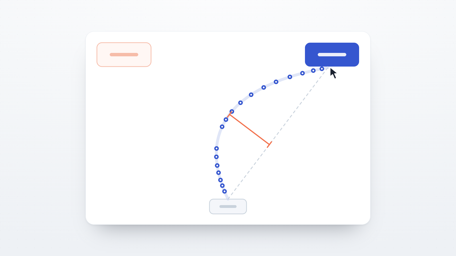
In a standard choice task, each trial yields a response and the time at which it was given. Mouse-tracking adds the path the cursor takes between the start of the trial and the click. If a participant moves toward one option before settling on the other, or curves toward the unchosen option on the way to the chosen one, the trajectory records it. Researchers use this record to study how strongly the response options compete while a decision is being made (Wulff et al., 2025).

Collecting these data online involves three steps: recording cursor positions in the browser, designing trials that produce interpretable trajectories, and reading the recorded positions into an analysis pipeline. This post covers each step for studies built in lab.js and run on Open Lab. In lab.js, cursor positions are recorded with the Mousetrap plugin, which the tutorial by Wulff et al. (2025) refers to as mousetrap-web, and the output can be analysed with the mousetrap R package (Kieslich & Henninger, 2017). The post describes what the plugin records, how it behaves on participants' own computers and phones, and which import settings its output needs.

The standard mouse-tracking trial

Most mouse-tracking studies use a layout established in early work on spoken-word recognition. In the study by Spivey, Grosjean and Knoblich (2005), participants clicked a box at the bottom centre of the screen, two pictures appeared in the upper left and right corners, and a spoken word such as "candle" followed 500 ms later. Participants then clicked the named picture. When the other picture showed an object with a similar-sounding name (a candy), cursor paths curved further toward it than when the other picture showed an unrelated object (a jacket). Freeman and Ambady (2010) made a similar layout the default in their MouseTracker software, with a start button at the bottom centre of the screen and the response options in the top corners.

A recorded trajectory is a series of time-stamped x and y coordinates. Several summary measures are computed from it:

• Maximum absolute deviation (MAD): the largest perpendicular distance between the trajectory and the straight line from its start point to its end point.
• Area under the curve (AUC): the area between the trajectory and that straight line.
• x-flips: the number of reversals of direction along the horizontal axis.
• Initiation time: the time from the start of the trial until the cursor begins to move.

Larger MAD and AUC values toward the unchosen option are interpreted as stronger attraction toward that option. Because trials differ in duration, trajectories are usually resampled into 101 time steps before they are averaged, which is the convention from Spivey et al. (2005) and the default in both MouseTracker and the mousetrap package (Freeman & Ambady, 2010; Wulff et al., 2025).

Design choices that change the trajectories

How a trial starts and how a response is given both affect the trajectories that are recorded.

Starting procedure. In a static start, the stimulus appears when the participant clicks the start button, or after a short fixed delay, and the participant may begin moving whenever they choose. In a dynamic start, the stimulus appears only once the participant has started moving the cursor upward. Scherbaum and Kieslich (2018) compared the two in a Simon task. With a static start, movements were less consistent, and the effects in measures taken within the trial were weaker and compressed into a shorter period. They recommend a dynamic start for studies that analyse how a trajectory develops over time. Their dynamic condition came from an earlier study, so participants were not randomly assigned to the two procedures. Kieslich, Schoemann, Grage, Hepp and Scherbaum (2020) randomly assigned 245 participants to one of four starting procedures in a typicality task, in which animals are sorted into one of two categories. The size of the typicality effect on MAD did not differ significantly between the static and the dynamic start, but the dynamic start produced mostly curved trajectories.

Response indication. A response can be given by clicking an option or by moving the cursor into the option's area without clicking. In the same set of experiments, the typicality effect on MAD was larger with clicks (dz = 0.61) than with this hover response (dz = 0.36). Clicks produced a mix of straight trajectories and trajectories that changed direction partway, while hover responses produced mostly straight trajectories (Kieslich et al., 2020). Grage, Schoemann, Kieslich and Scherbaum (2019) varied the response format, the ratio of cursor movement to hand movement and the position of the response boxes. They report that each of these factors can blur the relationship between the cognitive process and the movement, and they recommend clicks with a static start, hover responses with a dynamic start, and response boxes placed directly in the top corners.

Wulff et al. (2025) summarise these studies without prescribing a single setup. They note that designs producing larger effects tend to produce less homogeneous trajectories, and that the setup should be chosen with the theoretical background and the planned analyses in mind.

Recording cursor positions with the lab.js Mousetrap plugin

The Mousetrap plugin for lab.js was developed by the authors of lab.js and of the mousetrap package. It was added to the lab.js builder as a beta feature with lab.js 20.0.0 (Kieslich, 2020), and the current plugin file is version 0.1.0. In the builder, every component has a Plugins tab. To record trajectories, select the screen on which the response is given, open its Plugins tab, add Mousetrap, and choose a data format.

The plugin records from the moment the component it is attached to starts until that component ends. Attached to the response screen, it produces one trajectory per trial in that trial's data row. Movement made during an earlier screen is not recorded. Langridge and Marotta (2022), who used the plugin in three remote experiments, report that a coding error allowed participants to start moving during a 200 ms mask before the response screen, so that movement on 1.6% to 2.6% of trials was not captured.

The plugin offers two data formats:

• Mousetrap default adds four columns to the screen's data row. xpos and ypos hold the cursor positions in pixels, measured from the top left corner of the page, so ypos increases as the cursor moves down. timestamps holds the time of each sample in milliseconds. mouseouts holds the times of mouseout events.
• Event stream adds a single column, mouseData, with every recorded event (movements, button presses, releases and clicks) as an object that includes its type, time and coordinates.

Four properties of the plugin matter for the analysis.

1. Samples are recorded only when the cursor moves. The plugin adds a sample each time the browser reports a mousemove event. While the cursor is stationary, nothing is recorded. The first sample is therefore the first movement after the screen starts, not the starting position, and a pause appears as a gap between two timestamps. The mousetrap plugin for OpenSesame works differently: by default it records the cursor position every 10 ms, whether or not the cursor moves (Kieslich & Henninger, 2017).
2. The sampling rate depends on the browser and the display. Since version 60, Chrome aligns mousemove events to display frames: it holds them and delivers them immediately before the page draws the next frame, although a mouse typically reports its position about 100 times per second (Tapuska, 2017). On a 60 Hz display, a moving cursor is therefore sampled about every 16.7 ms. In an online study with a different browser-based tool, Mathur and Reichling (2019) observed a median interval of 17 ms between recorded positions. Other browsers and displays with higher refresh rates produce other intervals.
3. Timestamps share lab.js's clock. Each timestamp is the event's timeStamp, which is measured from the same origin as the time_run, time_show and time_end values that lab.js records for every screen (MDN Web Docs, n.d.-a). Browsers round these values to between 0.1 ms and 1 ms by default.
4. mouseouts is not a measure of leaving the window. A mouseout event fires whenever the cursor leaves any element on the page, including a button or a paragraph of text (MDN Web Docs, n.d.-b). The column therefore fills up during ordinary movement.

Elements marked with a data-mt attribute are handled separately. When the screen starts, the plugin records the label, position and size of each such element in a further column, mouseEnvironment. Marking the two response buttons this way records where they appeared on each participant's screen.

An example trial in lab.js

The example below uses two HTML screens inside the trial sequence of a loop, for an animal categorisation task. The loop's rows provide stimulus, left, right and correct for each trial, for example "whale", "fish", "mammal" and "right". The response labels are visible on both screens, so the layout does not change when the stimulus appears.

The start screen has the response "click button#start":

<button style="position: fixed; top: 2rem; left: 2rem; width: 10rem; height: 4rem;">${ parameters.left }</button>
<button style="position: fixed; top: 2rem; right: 2rem; width: 10rem; height: 4rem;">${ parameters.right }</button>
<button id="start" style="position: fixed; bottom: 2rem; left: 50%; transform: translateX(-50%); width: 8rem; height: 3rem;">Start</button>

The response screen carries the Mousetrap plugin. Its responses are "click button#left" → left and "click button#right" → right, and its correct response is ${ parameters.correct }:

<button id="left" data-mt="left" style="position: fixed; top: 2rem; left: 2rem; width: 10rem; height: 4rem;">${ parameters.left }</button>
<button id="right" data-mt="right" style="position: fixed; top: 2rem; right: 2rem; width: 10rem; height: 4rem;">${ parameters.right }</button>
<p style="position: fixed; bottom: 6rem; width: 100%; text-align: center; font-size: 2rem;">${ parameters.stimulus }</p>

Only the buttons with an id are mapped to responses, so clicking a label on the start screen has no effect. This is a static start. A dynamic start would need a script on the response screen that keeps the stimulus hidden until the cursor has moved a set distance upward from the start button.

Running the task on Open Lab

A task that uses the Mousetrap plugin is saved to Open Lab or uploaded in the same way as any other lab.js task. When Open Lab assembles the task, it includes the plugin, and the participant's browser loads the plugin file when the task starts. We checked this on the lab.js version that Open Lab uses to run tasks (20.2.4) by running the example above in an automated browser and moving the cursor along curved paths. Each response screen's row contained the four trajectory columns and mouseEnvironment, and no other row contained them.

The Individual responses (CSV) download in a study's Data view has one row per lab.js component, so each trial's response screen is one row. The trajectory columns contain the recorded values as text in JSON array notation, for example [487,476,468,…]. The post on the Data view and the Data Explorer describes the other export formats.

What changes when participants use their own devices

In a laboratory study, participants usually work with the same mouse, the same pointer settings and the same screen. Online, all three vary between participants. The paragraphs below describe which of these differences can be recorded in the data, which can be corrected in the analysis, and which can only be limited through the instructions.

Touchscreens produce no trajectory. The plugin listens for mouse events. When a browser treats a tap as a click, it sends a single sequence of mouse events at the point where the finger was lifted (W3C, 2013). We checked the plugin's behaviour in Chromium with touch emulation: dragging a finger from the start button to a response option recorded no samples, and the tap on the option recorded one. A trial with one sample or none was therefore most likely answered by touch. Open Lab does not restrict studies to particular device types, so the requirement for a computer with a mouse belongs in the study description and the instructions, and touch responses should be identified in the data.

The type of pointing device can be recorded with a short script. The following lines, added to the run event of an instruction screen, store whether the main pointing device is a fine one or a coarse one, and how many simultaneous touch points the device supports:

this.data.pointer_fine = window.matchMedia("(pointer: fine)").matches
this.data.any_hover = window.matchMedia("(any-hover: hover)").matches
this.data.max_touch_points = navigator.maxTouchPoints

The Media Queries specification lists mice, touchpads and drawing styluses as fine pointers and touchscreens as coarse ones (W3C, 2026), so this check separates touchscreens from the rest but does not separate a trackpad from a mouse.

Mice and trackpads produce different movements. Warburton, Campagnoli, Mon-Williams, Mushtaq and Morehead (2025) compared participants recruited on Prolific who used a mouse with those who used a trackpad in two online movement tasks. Reaction times were consistently higher for trackpad users, and other movement measures also differed between the devices. The authors recommend recording the input device in online experiments. The browser does not report it, so a question at the end of the study is the practical way to do so. Langridge and Marotta (2022) instead required all participants to use the trackpad of their own laptop, so that the device was the same for everyone.

Pointer speed and display scaling cannot be set by the study. Laboratory studies can fix the ratio of cursor movement to hand movement and switch off pointer acceleration, which Kieslich et al. (2020) recommend for simple tasks. Online, these settings belong to the participant's operating system, and a browser-based study cannot change them (Mathur & Reichling, 2019). Mathur and Reichling also found larger trajectory measures for participants whose pixel scaling was non-standard, for example because the page was zoomed, even after trajectories were rescaled. The main effect of their stimulus manipulation was present regardless. The lab.js Metadata plugin, added to the root of the study, records the window size, the screen size and the device pixel ratio for each session, so scaling can be included as a covariate or used for exclusions.

Window sizes differ. The positions of the buttons in the example depend on the size of the browser window, so the same movement covers a different number of pixels on different screens. The mouseEnvironment column records where the response buttons were on each trial. In the analysis, aligning all trajectories to a common start and end point removes differences in scale (see the next section). Very small windows can be excluded, or participants can be asked to maximise the window before the task starts.

Sampling intervals differ. Time normalisation makes trajectories with different sampling rates comparable for averaging, and Wulff et al. (2025) describe resampling as a way to handle the variable sampling rates that are common in browser-based tracking. Neither step recovers movement between two samples. The mousetrap function mt_check_resolution() summarises the intervals between samples, and Langridge and Marotta (2022) used it to check the logging resolution of each dataset.

Reading the export into the mousetrap R package

Wulff et al. (2025) describe the full preprocessing and analysis sequence in the mousetrap package. The plugin's output can be read with mt_import_mousetrap(), which accepts the JSON-style arrays in the CSV without further conversion. One import setting needs attention. By default, the import sets the first timestamp of every trial to zero, on the assumption that the first sample marks the start of recording. That assumption holds for the OpenSesame plugin, which records from the start of the trial. Because the lab.js plugin records nothing until the cursor moves, its first sample marks the first movement. With the default setting, every initiation time would be zero, and the response time would cover the movement only.

The code below keeps the original timestamps and subtracts time_run instead: the time at which the response screen started and the plugin began listening. It assumes the response screen is named "Response" in the builder; the sender column contains each screen's name.

library(mousetrap)

raw <- read.csv("individual_responses.csv")
trials <- subset(raw, sender == "Response")

# Trials answered by touch contain one sample or none
trials$n_samples <- lengths(strsplit(trials$xpos, ","))
trials <- subset(trials, n_samples > 1)

mt <- mt_import_mousetrap(trials, reset_timestamps = FALSE)

# Time zero: the response screen started and the plugin began recording
mt$trajectories[, , "timestamps"] <-
  mt$trajectories[, , "timestamps"] - mt$data$time_run

mt_check_resolution(mt)$summary   # intervals between samples, in ms

mt <- mt_align_start_end(mt)   # every trajectory starts at (0, 0) and ends at (-1, 1)
mt <- mt_time_normalize(mt)    # 101 time steps per trajectory
mt <- mt_measures(mt)          # MAD, AUC, x-flips, RT, initiation time, ...

agg <- mt_aggregate(mt, use = "measures",
                    use_variables = c("MAD", "AUC", "RT"),
                    use2_variables = "correct",
                    subject_id = "Participant.Code")

Several details of this code follow from the plugin's behaviour.

• time_show, the time at which the screen was first displayed, is not used as time zero. A participant who is already moving when the stimulus appears produces samples a few milliseconds before time_show, and mt_measures() stops with an error when a trajectory starts before zero. time_run precedes time_show by about one frame, so response times computed this way are slightly longer than lab.js's own duration column, which is counted from time_show.
• With time_run as zero, mt_measures() prints a note that some trajectories start after timestamp 0. This is expected here, because the first sample is the first movement.
• mt_align_start_end() rescales each trajectory so that it starts at (0, 0) and ends at (−1, 1). This removes differences in window size and places responses to the left and to the right option on the same side, so that deviations toward the unchosen option have the same sign for both. The package's mt_remap_symmetric() assumes a coordinate system centred on the screen, whereas browser coordinates start at the top left corner of the page, so it is not used here.
• Measures of pausing, such as hover_time and idle_time, need regularly spaced samples. Because a pause produces no samples, it is not detected in the raw data. Resampling with constant interpolation across longer gaps, for example mt_resample(mt, step_size = 10, constant_interpolation = 100), fills a pause with the last recorded position before these measures are computed. In a test with a simulated 400 ms pause, hover_time was 0 without this step and 350 ms with it.

We ran this code on a CSV in Open Lab's export format, produced by the automated browser run described above with two simulated mouse users and one touchscreen user. The touchscreen trials were removed by the sample count, and the import, alignment, time normalisation and measures ran without changes. In a separate test, MAD and AUC were unchanged after all coordinates were scaled by a factor of 1.5, as they would be on a larger window.

What to report

Schoemann, O'Hora, Dale and Scherbaum (2021) reviewed 167 mouse-tracking experiments and found that only 1.81% reported all eight design features they examined precisely. They propose a minimal reporting standard that includes the input device, the monitor's resolution and size, cursor speed and acceleration, the size and position of the start and response areas, the starting and response procedures, the sampling rate, the normalisation applied, and the setting in which the data were collected.

In an online study, several of these features vary between participants and are better reported as recorded values or distributions than as a single setting. The methods section can state the lab.js and plugin versions and the data format, the device requirement and how it was communicated, how touch responses and very small windows were identified and excluded, the distribution of window sizes and pixel ratios, the self-reported input devices, and the distribution of sampling intervals. The lab.js task file, exported as JSON, can be shared with the study materials so that the trial layout and starting procedure can be reproduced exactly.